[그래프 신경망과 빅데이터] GAE 모델을 활용한 소셜 네트워크 링크 예측 및 이상치 탐지

ML, DL, GNN 비교하기

1. 머신러닝 (Machine Learning, ML): "기본 레시피"

• 개념:
  - 가장 넓은 개념으로, 컴퓨터가 데이터로부터 스스로 학습하게 만드는 모든 기술을 말함
• 특징:
  - 개발자가 직접 재료(데이터)의 특징(Feature)을 손질해야 함
  - 예를 들어, 집값을 예측하는 모델을 만들 때 "방의 개수", "평수", "지하철역과의 거리"와 같이 어떤 특징이 중요한지를 사람이 직접 선택하고 가공하여 모델에게 알려줘야 함
• 비유:
  - 기본적인 **"레시피"**와 같음
  - 레시피에 적힌 재료와 순서대로 요리를 만들면 어느 정도 맛있는 음식을 만들 수 있음

## 2. 딥러닝 (Deep Learning, DL): "스스로 재료를 고르는 셰프"

• 개념:
  - 머신러닝의 한 분야로, 인간의 뇌 신경망을 모방한 인공 신경망을 깊게(Deep) 쌓아 올려 학습하는 기술
• 특징:
  - 딥러닝의 가장 큰 혁신은 "특징 추출(Feature Extraction)"을 자동화했다는 점
  - 개발자가 어떤 특징이 중요한지 일일이 알려주지 않아도, 모델이 방대한 데이터(예: 수백만 장의 강아지 사진)를 보고 "강아지"를 구별하는 최적의 특징(뾰족한 귀, 털의 질감 등)을 스스로 학습
• 비유:
  - 수많은 식재료를 보고 최상의 조합을 스스로 찾아내는 **"최고의 셰프"**와 같음
  - 셰프는 레시피 없이도, 재료 본연의 맛과 향을 스스로 파악하여 최고의 요리를 만들어냄

## 3. 그래프 신경망 (Graph Neural Network, GNN): "재료 간의 '궁합'을 보는 셰프"

• 개념:
  - 딥러닝의 한 종류로, '관계'를 학습하는 데 특화된 기술
• 특징:
  - 기존 딥러닝 모델들이 이미지나 텍스트처럼 각각의 데이터가 독립적이라고 가정하는 반면, GNN은 데이터 간의 '관계'와 '연결 구조' 자체를 핵심 정보로 활용
• 비유:
  - 재료 하나하나의 맛뿐만 아니라, **재료들 사이의 '궁합'**까지 고려하여 요리하는 셰프와 같음"
  - 이 허브는 이 생선과 어울리고, 저 소스는 이 야채와 만났을 때 최고의 맛을 낸다"와 같이, 개체(노드)와 그들 사이의 관계(엣지)를 함께 학습하여 전체 요리의 조화를 완성

---

1단계: 데이터 준비 - 모델을 위한 교과서와 시험지 만들기

• 스탠포드 대학교에서 제공하는 ego-Facebook 데이터셋을 사용(아래의 링크에서 'facebook_combined.txt' 다운)
  - https://snap.stanford.edu/data/ego-Facebook.html
• 이 데이터는 4,039명의 사용자와 그들 사이의 88,234개 친구 관계를 담고 있음
• .txt 파일을 .csv 파일로 변환 먼저, 다루기 쉽도록 원본 .txt 파일을 .csv 파일로 변환

SNAP: Network datasets: Social circles

# .txt → .csv

import pandas as pd

# 파일 경로
txt_file_path = 'facebook_combined.txt'
csv_file_path = 'facebook_combined.csv'

# txt 파일 읽어옴. 공백으로 열이 구분되어 있고, 헤더는 없습니다.
# names=['source', 'target'] 으로 각 열에 이름을 붙여줌.
edge_list = pd.read_csv(txt_file_path, sep=' ', header=None, names=['source', 'target'])

# DataFrame을 CSV 파일로 저장
# index=False 옵션은 맨 앞의 번호(인덱스)를 저장하지 않도록 함.
edge_list.to_csv(csv_file_path, index=False)

print(f"'{csv_file_path}' 파일이 성공적으로 생성!")

# PyTorch의 Tensor라는 데이터 형식으로 저장되어 있는 것.
# edge_index: 모델이 구조를 학습할 '불완전한 그래프'의 엣지 정보이다. (훈련용)
# edge_label_index: 모델이 "이 둘은 친구일까 아닐까?" 하고 풀어야 할 '문제지'이다. 여기에는 숨겨놓은 진짜 엣지(Positive)와 우리가 찾고 있는 가짜 엣지(Negative)가 모두 들어있다.
# edge_label: 바로 위 edge_label_index에 대한 '정답지'이다. 각 엣지가 진짜면 1, 가짜면 0이라는 값을 가진다.

import pandas as pd
import torch
import torch.nn as nn
import torch.nn.functional as F
from torch_geometric.data import Data
from torch_geometric.transforms import RandomLinkSplit
from torch_geometric.nn import GCNConv, GAE
import matplotlib.pyplot as plt
from sklearn.metrics import roc_auc_score, average_precision_score
import random
import numpy as np

seed = 42
random.seed(seed)
np.random.seed(seed)
torch.manual_seed(seed)

# 1. 원본 엣지 리스트 불러오기
file_path = 'facebook_combined.csv' # (2, 88,234)
edge_list = pd.read_csv(file_path)
edge_index = torch.tensor(edge_list.values).t().contiguous()

# 2. PyG 그래프 데이터 객체 생성
# 전체 엣지 정보를 담은 '원본 그래프'를 만든다.
data = Data(edge_index=edge_index)

# 3. 데이터 분할을 위한 변환(Transform) 정의
# is_undirected=True: 무방향 그래프임을 명시 (A-B 친구면 B-A도 친구)
# add_negative_train_samples=True: 훈련 세트에 1:1 비율로 가짜 엣지 자동 추가
# neg_sampling_ratio=1.0: 검증/테스트 세트에도 1:1 비율로 가짜 엣지 자동 추가
transform = RandomLinkSplit(
    num_val=0.05,  # 검증(Validation) 세트 비율: 5%
    num_test=0.10, # 시험(Test) 세트 비율: 10%
    is_undirected=True,
    add_negative_train_samples=True,
    neg_sampling_ratio=1.0
)

# 4. '원본 그래프'에 transform을 적용하여 데이터 분할 실행
# 이 한 줄로 훈련/검증/시험용 엣지 분리 및 가짜 엣지 생성이 모두 끝.
train_data, val_data, test_data = transform(data)

# --- 결과 확인 ---
print("--- 분할 결과 ---")
print(f"훈련용 데이터셋 (Train Data):\n{train_data}\n")
print(f"검증용 데이터셋 (Validation Data):\n{val_data}\n")
print(f"시험용 데이터셋 (Test Data):\n{test_data}")
print("-" * 20)
print("각 세트의 엣지 정보를 자세히 살펴볼까요?")
print(f"[훈련 세트] 실제 엣지 수: {train_data.edge_label_index.shape[1] // 2}") # 85%
print(f"          가짜 엣지 수: {train_data.edge_label_index.shape[1] - train_data.edge_label.sum().int().item()}")
print(f"          (모델이 학습할 불완전한 그래프의 엣지 수: {train_data.edge_index.shape[1]})")
print("-" * 20)
print(f"[검증 세트] 실제 엣지 수: {val_data.edge_label.sum().int().item()}") # 5%
print(f"          가짜 엣지 수: {val_data.edge_label_index.shape[1] - val_data.edge_label.sum().int().item()}")
print("-" * 20)
print(f"[테스트 세트] 실제 엣지 수: {test_data.edge_label.sum().int().item()}") # 10%
print(f"           가짜 엣지 수: {test_data.edge_label_index.shape[1] - test_data.edge_label.sum().int().item()}\n")

# --- 가짜 엣지 데이터 직접 확인해보기(val_data) ---
val_edges_to_predict = val_data.edge_label_index
val_answers = val_data.edge_label

print("--- 검증용(val) 데이터 내부 확인 ---")
print(f"모델이 풀어야 할 전체 문제 (edge_label_index):\n{val_edges_to_predict}")
print(f"각 문제에 대한 정답 (edge_label):\n{val_answers}")
print("-" * 30)

# 2. '정답지'를 보고 정답이 0인 문제, 즉 '가짜 엣지'만 골라냄.
# val_answers가 0인 위치(인덱스)를 찾음.
negative_edge_indices = (val_answers == 0).nonzero(as_tuple=True)[0]

# 해당 위치에 있는 '가짜 엣지'들만 `edge_label_index`에서 추출.
negative_edges = val_edges_to_predict[:, negative_edge_indices]

print(f"찾았다! '가짜 엣지' 데이터:\n{negative_edges}")
print(f"\n총 {negative_edges.shape[1]}개의 가짜 엣지가 여기에 들어있습니다.")

• 모델을 가르치고, 평가하기 모델을 똑똑하게 만들려면, 공부할 교과서와 잘 배웠는지 테스트할 시험지가 필요
• RandomLinkSplit이라는 도구를 사용해 원본 데이터를 세 부분으로 나눔
  • 훈련(Train) 세트 (85%): 모델이 공부할 교과서. 일부러 몇몇 친구 관계를 숨겨놓은 "불완전한" 관계도
  • 검증(Validation) 세트 (5%): 모델이 공부하는 중간중간 보게 될 중간고사. 과적합을 방지하고 최적의 학습 시점을 찾기 위해 사용
  • 테스트(Test) 세트 (10%): 모든 학습이 끝난 뒤, 모델의 최종 실력을 평가할 기말고사

import torch
from torch_geometric.data import Data
from torch_geometric.transforms import RandomLinkSplit

# 랜덤 시드 고정으로 매번 같은 데이터셋을 생성
seed = 42
random.seed(seed)
np.random.seed(seed)
torch.manual_seed(seed)

# ... 데이터 로딩 ...

# 3. 데이터 분할을 위한 변환(Transform) 정의
transform = RandomLinkSplit(
    num_val=0.05,
    num_test=0.10,
    is_undirected=True,
    add_negative_train_samples=True, # "친구가 아닌 관계"도 학습 데이터에 추가
    neg_sampling_ratio=1.0
)

# 4. '원본 그래프'에 transform을 적용하여 데이터 분할 실행
train_data, val_data, test_data = transform(data)

 

add_negative_train_samples=True 옵션

- 모델에게 "누가 친구인지"만 학습하면 모든 사람을 친구라고 예측할 수 있음
- "누가 친구가 아닌지"도 함께 학습해야 진짜 친구 관계의 패턴을 정확히 배울 수 있음

---

2단계: GNN 모델 설계 - 관계를 학습할 두뇌 만들기

• 핵심 엔진은 **그래프 오토인코더(Graph Autoencoder, GAE)**
• GAE는 두 부분으로 이루어져 있음
  • 인코더 (Encoder):
    - 그래프의 복잡한 구조를 보고, 각 사용자의 사회적 특징을 '임베딩'이라는 작은 벡터로 똑똑하게 요약하는 역할을 함
  • 디코더 (Decoder):
    - 인코더가 만든 요약본(임베딩)만 보고, 원래의 친구 관계를 **복원(예측)**하는 역할을 함

2개의 GCN(그래프 합성곱 신경망) 레이어를 가진 인코더를 설계

• 1차 GCN 레이어: 각 사용자가 자신의 직접적인 친구들의 정보를 수집
• 2차 GCN 레이어: 친구들이 수집한 정보를 다시 전달받아, '친구의 친구' 정보까지 종합하여 최종 프로필(임베딩)을 완성

import torch.nn as nn

# 하이퍼파라미터 (Optuna로 찾은 최적값)
latent_dim = 112
num_layers = 2
dropout_rate = 0.337
learning_rate = 0.0087
weight_decay = 1.36e-05

# 2. GAE 모델 정의
class GCNEncoder(nn.Module):
    def __init__(self, in_channels, hidden_channels, out_channels, num_layers, dropout):
        super().__init__()
        self.convs = nn.ModuleList()
        self.convs.append(GCNConv(in_channels, hidden_channels))
        for _ in range(num_layers - 2):
            self.convs.append(GCNConv(hidden_channels, hidden_channels))
        self.convs.append(GCNConv(hidden_channels, out_channels))
        self.dropout = dropout

    def forward(self, x, edge_index):
        for i, conv in enumerate(self.convs):
            x = conv(x, edge_index)
            if i != len(self.convs) - 1:
                x = x.relu()
                x = F.dropout(x, p=self.dropout, training=self.training)
        return x

# 모델 및 옵티마이저 생성
encoder = GCNEncoder(in_channels, 2 * latent_dim, latent_dim, num_layers, dropout_rate)
model = GAE(encoder)
optimizer = torch.optim.Adam(model.parameters(), lr=learning_rate, weight_decay=weight_decay)

 

• 사람-사람의 데이터 셋은 동종 그래프에 해당하기 때문에, GAE 모델을 사용함
• 사람-상품과 같은 이분 그래프에서는 LigtjGCN 모델을 사용하는 것이 더 적합함

최적의 하이퍼파라메터 튜닝을 위해, Optuna 라이브러리를 사용하여 50개의 trial을 실험하여 최적의 값을 찾아냄

# 최적 파라메터 찾기
# ---------------------------------------------------
# 0. Optuna 설치
# ---------------------------------------------------
!pip install optuna

import optuna
import pandas as pd
import torch
import torch.nn as nn
import torch.nn.functional as F
from torch_geometric.data import Data
from torch_geometric.transforms import RandomLinkSplit
from torch_geometric.nn import GCNConv, GAE
from sklearn.metrics import roc_auc_score

# ---------------------------------------------------
# 1. 데이터 준비 (전역 변수로 한 번만 로딩)
# ---------------------------------------------------
file_path = 'facebook_combined.txt'
edge_list = pd.read_csv(file_path, sep=' ', header=None, names=['source', 'target'])
edge_index = torch.tensor(edge_list.values).t().contiguous()
num_nodes = edge_index.max().item() + 1
data = Data(edge_index=edge_index, num_nodes=num_nodes)
transform = RandomLinkSplit(
    num_val=0.05, num_test=0.10, is_undirected=True,
    add_negative_train_samples=True, neg_sampling_ratio=1.0
)
train_data, val_data, test_data = transform(data)
x = F.one_hot(torch.arange(num_nodes)).float()
in_channels = x.size(1)

# ---------------------------------------------------
# 2. "objective" 함수 정의: 모델 학습 및 평가 전체 과정
# ---------------------------------------------------
def objective(trial):
    # --- A. 하이퍼파라미터 탐색 범위 설정 ---
    latent_dim = trial.suggest_int('latent_dim', 32, 128, step=16) # 32, 48, 64...
    num_layers = trial.suggest_int('num_layers', 2, 4)
    dropout_rate = trial.suggest_uniform('dropout_rate', 0.2, 0.6)
    learning_rate = trial.suggest_loguniform('learning_rate', 1e-3, 1e-2) # 0.001 ~ 0.01
    weight_decay = trial.suggest_loguniform('weight_decay', 1e-5, 1e-3)

    # --- B. 모델 정의 및 학습 (기존 코드와 거의 동일) ---
    class GCNEncoder(nn.Module):
        def __init__(self, in_channels, hidden_channels, out_channels, num_layers, dropout):
            super().__init__()
            self.convs = nn.ModuleList()
            self.convs.append(GCNConv(in_channels, hidden_channels))
            for _ in range(num_layers - 2):
                self.convs.append(GCNConv(hidden_channels, hidden_channels))
            self.convs.append(GCNConv(hidden_channels, out_channels))
            self.dropout = dropout

        def forward(self, x, edge_index):
            for i, conv in enumerate(self.convs):
                x = conv(x, edge_index)
                if i != len(self.convs) - 1:
                    x = x.relu()
                    x = F.dropout(x, p=self.dropout, training=self.training)
            return x

    encoder = GCNEncoder(in_channels, 2 * latent_dim, latent_dim, num_layers, dropout_rate)
    model = GAE(encoder)
    optimizer = torch.optim.Adam(model.parameters(), lr=learning_rate, weight_decay=weight_decay)

    # 학습 루프
    epochs = 200 # 최적화 중에는 에포크를 줄여서 빠르게 테스트
    for epoch in range(1, epochs + 1):
        model.train()
        optimizer.zero_grad()
        z = model.encode(x, train_data.edge_index)
        loss = model.recon_loss(z, train_data.edge_index)
        loss.backward()
        optimizer.step()

    # --- C. 성능 평가 및 목표 점수 반환 ---
    model.eval()
    with torch.no_grad():
        z = model.encode(x, val_data.edge_index)
        preds = model.decode(z, val_data.edge_label_index).sigmoid()
        labels = val_data.edge_label
        val_auc = roc_auc_score(labels.cpu(), preds.cpu())

    # Optuna는 이 점수를 최대화하는 방향으로 다음 하이퍼파라미터를 탐색
    return val_auc

# ---------------------------------------------------
# 3. Study 생성 및 최적화 실행
# ---------------------------------------------------
# "maximize" a Val AUC score
study = optuna.create_study(direction='maximize')
# 50번의 다른 하이퍼파라미터 조합으로 실험
study.optimize(objective, n_trials=50) # 50번의 trial 실행

# ---------------------------------------------------
# 4. 결과 확인
# ---------------------------------------------------
print("\n--- Optuna 하이퍼파라미터 최적화 완료 ---")
print(f"총 실험 횟수: {len(study.trials)}")
print(f"최고의 Val AUC 점수: {study.best_value:.4f}")
print("최적의 하이퍼파라미터 조합:")
for key, value in study.best_params.items():
    print(f"  - {key}: {value}")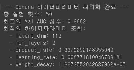

---

3단계: 학습 및 평가 - AI를 학습시키기

• 모델은 교과서(train_data.edge_index)를 보고 친구 관계의 패턴을 학습하고, 중간고사(val_data)를 보며 학습 방향을 점검

# ---------------------------------------------------
# 3. 모델 학습 루프
# ---------------------------------------------------
loss_history = []
def train():
    model.train()
    optimizer.zero_grad()
    z = model.encode(x, train_data.edge_index)
    # loss = model.recon_loss(z, train_data.edge_label_index)
    loss = model.recon_loss(z, train_data.edge_index)
    loss.backward()
    optimizer.step()
    return float(loss.detach()) # .detach()를 추가하여 경고 메시지 해결

# ---------------------------------------------------
# 4. 모델 성능 테스트 함수 (오류 수정)
# ---------------------------------------------------
@torch.no_grad()
def test(data_split):
    model.eval()
    z = model.encode(x, data_split.edge_index)

    # 1. '문제지(edge_label_index)'에 대한 모델의 예측값(확률)을 얻음
    preds = model.decode(z, data_split.edge_label_index).sigmoid()
    # 2. '정답지(edge_label)'를 가져옴
    labels = data_split.edge_label

    # 3. 예측값과 정답지를 비교하여 성능 점수(AUC, AP) 계산
    auc = roc_auc_score(labels.cpu(), preds.cpu())
    ap = average_precision_score(labels.cpu(), preds.cpu())

    return auc, ap

# ---------------------------------------------------
# 5. 실제 학습 및 평가 실행
# ---------------------------------------------------
for epoch in range(1, epochs + 1):
    loss = train()
    loss_history.append(loss)
    if epoch % 10 == 0:
        val_auc, val_ap = test(val_data)
        print(f'Epoch: {epoch:03d}, Loss: {loss:.4f}, Val AUC: {val_auc:.4f}, Val AP: {val_ap:.4f}')

test_auc, test_ap = test(test_data)
print("-" * 30)
print(f'최종 성능 => Test AUC: {test_auc:.4f}, Test AP: {test_ap:.4f}') # AUC: 분별력 점수, AP: 정확성 점수 -> 1에 가까울 수록 똑똑한 모델


# ---------------------------------------------------
# 6. Loss 그래프 그리기
# ---------------------------------------------------
plt.figure(figsize=(10, 6))
plt.plot(range(1, epochs + 1), loss_history, label='Training Loss')
plt.title('Training Loss Over Epochs')
plt.xlabel('Epochs')
plt.ylabel('Loss')
plt.legend()
plt.grid(True)
plt.savefig('loss_graph.png')
plt.show()
print("\n'loss_graph.png' 파일이 저장되었습니다.")

 

• 위 그래프처럼, 학습 초반에 오답률(Loss)이 급격히 감소하다가 잠시 정체기를 거쳐 다시 한번 감소하는 모습을 보임
• 이는 모델이 쉬운 패턴을 먼저 학습한 뒤, 더 복잡하고 미묘한 패턴까지 성공적으로 학습했다는 아주 긍정적인 신호
• 모든 학습이 끝난 뒤, **"기말고사(test_data)"**로 최종 성능을 평가한 결과는 다음과 같음

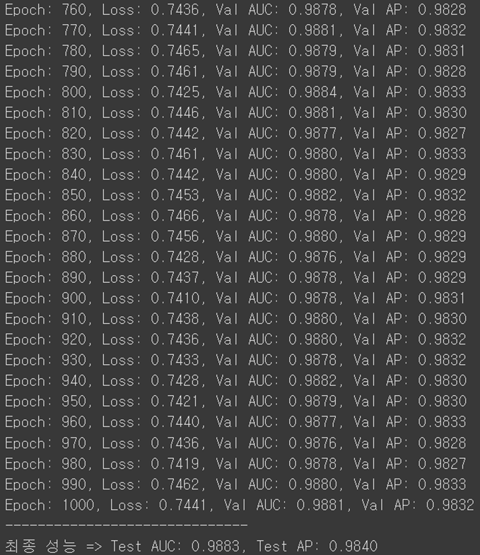
• AUC와 AP는 모델의 성능 점수로, 1에 가까울수록 완벽하다는 뜻
• 약 99%의 정확도로 숨겨진 친구 관계를 예측할 수 있는, 아주 똑똑한 모델이 만들어짐

---

4단계: 활용 - 친구 추천과 광고 봇 탐지

활용 1: 친구 추천 시스템

• 특정 사용자(예: 728번)에게 새로운 친구를 추천해 보았음
• 모델이 만든 임베딩 벡터를 기준으로, 728번 사용자와 가장 유사한 취향과 사회적 위치를 가진 사용자를 찾아내는 방식
• 결과를 검증하기 위해, 추천된 사용자와 728번 사용자가 **'공동 친구'**를 몇 명이나 가졌는지 확인해 보았음

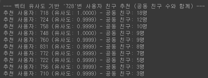
• 결과를 보니, 벡터 유사도가 높게 나온 사용자일수록 실제로도 공동 친구가 많은 경향을 보였음
• 이는 모델이 그래프의 구조를 정확히 이해하여, 같은 커뮤니티에 속한 잠재적 친구를 성공적으로 찾아냈음을 의미

활용 2: 이상치 탐지 (광고/스팸 봇 탐지)

• GAE 모델의 또 다른 강력한 기능은 이상치 탐지
• 모델은 대다수 '정상' 사용자의 패턴을 학습했기 때문에, 이 패턴에서 크게 벗어나는 사용자를 쉽게 찾아낼 수 있음
• '복원 오차(Reconstruction Error)'를 이상 점수로 사용 모델이 특정 사용자의 친구 관계를 제대로 복원하지 못할수록, 그 사용자는 비정상적일 확률이 높음
• 통계적 기준(평균 + 2 * 표준편차)을 적용하여 이상치를 탐지한 결과는 다음과 같음

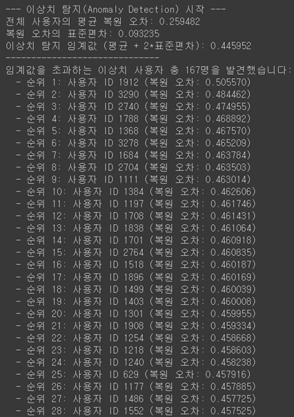
• 탐지된 사용자들은 일반 사용자와 달리, 전체 네트워크와는 고립된 채 무분별한 연결 패턴을 보이는 경향이 있었음
• 이는 이들이 광고나 스팸을 위한 봇 계정일 가능성이 높음을 시사

---

전체 코드

# .txt → .csv

import pandas as pd

# 파일 경로
txt_file_path = 'facebook_combined.txt'
csv_file_path = 'facebook_combined.csv'

# txt 파일 읽어옴. 공백으로 열이 구분되어 있고, 헤더는 없습니다.
# names=['source', 'target'] 으로 각 열에 이름을 붙여줌.
edge_list = pd.read_csv(txt_file_path, sep=' ', header=None, names=['source', 'target'])

# DataFrame을 CSV 파일로 저장
# index=False 옵션은 맨 앞의 번호(인덱스)를 저장하지 않도록 함.
edge_list.to_csv(csv_file_path, index=False)

print(f"'{csv_file_path}' 파일이 성공적으로 생성!")

#-----------------------------------------------------------------------------------------
!pip install torch
!pip install torch-geometric
!pip install matplotlib

# PyTorch의 Tensor라는 데이터 형식으로 저장되어 있는 것.
# edge_index: 모델이 구조를 학습할 '불완전한 그래프'의 엣지 정보이다. (훈련용)
# edge_label_index: 모델이 "이 둘은 친구일까 아닐까?" 하고 풀어야 할 '문제지'이다. 여기에는 숨겨놓은 진짜 엣지(Positive)와 우리가 찾고 있는 가짜 엣지(Negative)가 모두 들어있다.
# edge_label: 바로 위 edge_label_index에 대한 '정답지'이다. 각 엣지가 진짜면 1, 가짜면 0이라는 값을 가진다.

import pandas as pd
import torch
import torch.nn as nn
import torch.nn.functional as F
from torch_geometric.data import Data
from torch_geometric.transforms import RandomLinkSplit
from torch_geometric.nn import GCNConv, GAE
import matplotlib.pyplot as plt
from sklearn.metrics import roc_auc_score, average_precision_score
import random
import numpy as np

seed = 42
random.seed(seed)
np.random.seed(seed)
torch.manual_seed(seed)

# 1. 원본 엣지 리스트 불러오기
file_path = 'facebook_combined.csv' # (2, 88,234)
edge_list = pd.read_csv(file_path)
edge_index = torch.tensor(edge_list.values).t().contiguous()

# 2. PyG 그래프 데이터 객체 생성
# 전체 엣지 정보를 담은 '원본 그래프'를 만든다.
data = Data(edge_index=edge_index)

# 3. 데이터 분할을 위한 변환(Transform) 정의
# is_undirected=True: 무방향 그래프임을 명시 (A-B 친구면 B-A도 친구)
# add_negative_train_samples=True: 훈련 세트에 1:1 비율로 가짜 엣지 자동 추가
# neg_sampling_ratio=1.0: 검증/테스트 세트에도 1:1 비율로 가짜 엣지 자동 추가
transform = RandomLinkSplit(
    num_val=0.05,  # 검증(Validation) 세트 비율: 5%
    num_test=0.10, # 시험(Test) 세트 비율: 10%
    is_undirected=True,
    add_negative_train_samples=True,
    neg_sampling_ratio=1.0
)

# 4. '원본 그래프'에 transform을 적용하여 데이터 분할 실행
# 이 한 줄로 훈련/검증/시험용 엣지 분리 및 가짜 엣지 생성이 모두 끝.
train_data, val_data, test_data = transform(data)

# --- 결과 확인 ---
print("--- 분할 결과 ---")
print(f"훈련용 데이터셋 (Train Data):\n{train_data}\n")
print(f"검증용 데이터셋 (Validation Data):\n{val_data}\n")
print(f"시험용 데이터셋 (Test Data):\n{test_data}")
print("-" * 20)
print("각 세트의 엣지 정보를 자세히 살펴볼까요?")
print(f"[훈련 세트] 실제 엣지 수: {train_data.edge_label_index.shape[1] // 2}") # 85%
print(f"          가짜 엣지 수: {train_data.edge_label_index.shape[1] - train_data.edge_label.sum().int().item()}")
print(f"          (모델이 학습할 불완전한 그래프의 엣지 수: {train_data.edge_index.shape[1]})")
print("-" * 20)
print(f"[검증 세트] 실제 엣지 수: {val_data.edge_label.sum().int().item()}") # 5%
print(f"          가짜 엣지 수: {val_data.edge_label_index.shape[1] - val_data.edge_label.sum().int().item()}")
print("-" * 20)
print(f"[테스트 세트] 실제 엣지 수: {test_data.edge_label.sum().int().item()}") # 10%
print(f"           가짜 엣지 수: {test_data.edge_label_index.shape[1] - test_data.edge_label.sum().int().item()}\n")

# --- 가짜 엣지 데이터 직접 확인해보기(val_data) ---
val_edges_to_predict = val_data.edge_label_index
val_answers = val_data.edge_label

print("--- 검증용(val) 데이터 내부 확인 ---")
print(f"모델이 풀어야 할 전체 문제 (edge_label_index):\n{val_edges_to_predict}")
print(f"각 문제에 대한 정답 (edge_label):\n{val_answers}")
print("-" * 30)

# 2. '정답지'를 보고 정답이 0인 문제, 즉 '가짜 엣지'만 골라냄.
# val_answers가 0인 위치(인덱스)를 찾음.
negative_edge_indices = (val_answers == 0).nonzero(as_tuple=True)[0]

# 해당 위치에 있는 '가짜 엣지'들만 `edge_label_index`에서 추출.
negative_edges = val_edges_to_predict[:, negative_edge_indices]

print(f"찾았다! '가짜 엣지' 데이터:\n{negative_edges}")
print(f"\n총 {negative_edges.shape[1]}개의 가짜 엣지가 여기에 들어있습니다.")
#-----------------------------------------------------------------------------------------
# # 최적 파라메터 찾기
# # ---------------------------------------------------
# # 0. Optuna 설치
# # ---------------------------------------------------
# !pip install optuna

# import optuna
# import pandas as pd
# import torch
# import torch.nn as nn
# import torch.nn.functional as F
# from torch_geometric.data import Data
# from torch_geometric.transforms import RandomLinkSplit
# from torch_geometric.nn import GCNConv, GAE
# from sklearn.metrics import roc_auc_score

# # ---------------------------------------------------
# # 1. 데이터 준비 (전역 변수로 한 번만 로딩)
# # ---------------------------------------------------
# file_path = 'facebook_combined.txt'
# edge_list = pd.read_csv(file_path, sep=' ', header=None, names=['source', 'target'])
# edge_index = torch.tensor(edge_list.values).t().contiguous()
# num_nodes = edge_index.max().item() + 1
# data = Data(edge_index=edge_index, num_nodes=num_nodes)
# transform = RandomLinkSplit(
#     num_val=0.05, num_test=0.10, is_undirected=True,
#     add_negative_train_samples=True, neg_sampling_ratio=1.0
# )
# train_data, val_data, test_data = transform(data)
# x = F.one_hot(torch.arange(num_nodes)).float()
# in_channels = x.size(1)

# # ---------------------------------------------------
# # 2. "objective" 함수 정의: 모델 학습 및 평가 전체 과정
# # ---------------------------------------------------
# def objective(trial):
#     # --- A. 하이퍼파라미터 탐색 범위 설정 ---
#     latent_dim = trial.suggest_int('latent_dim', 32, 128, step=16) # 32, 48, 64...
#     num_layers = trial.suggest_int('num_layers', 2, 4)
#     dropout_rate = trial.suggest_uniform('dropout_rate', 0.2, 0.6)
#     learning_rate = trial.suggest_loguniform('learning_rate', 1e-3, 1e-2) # 0.001 ~ 0.01
#     weight_decay = trial.suggest_loguniform('weight_decay', 1e-5, 1e-3)

#     # --- B. 모델 정의 및 학습 (기존 코드와 거의 동일) ---
#     class GCNEncoder(nn.Module):
#         def __init__(self, in_channels, hidden_channels, out_channels, num_layers, dropout):
#             super().__init__()
#             self.convs = nn.ModuleList()
#             self.convs.append(GCNConv(in_channels, hidden_channels))
#             for _ in range(num_layers - 2):
#                 self.convs.append(GCNConv(hidden_channels, hidden_channels))
#             self.convs.append(GCNConv(hidden_channels, out_channels))
#             self.dropout = dropout

#         def forward(self, x, edge_index):
#             for i, conv in enumerate(self.convs):
#                 x = conv(x, edge_index)
#                 if i != len(self.convs) - 1:
#                     x = x.relu()
#                     x = F.dropout(x, p=self.dropout, training=self.training)
#             return x

#     encoder = GCNEncoder(in_channels, 2 * latent_dim, latent_dim, num_layers, dropout_rate)
#     model = GAE(encoder)
#     optimizer = torch.optim.Adam(model.parameters(), lr=learning_rate, weight_decay=weight_decay)

#     # 학습 루프
#     epochs = 200 # 최적화 중에는 에포크를 줄여서 빠르게 테스트
#     for epoch in range(1, epochs + 1):
#         model.train()
#         optimizer.zero_grad()
#         z = model.encode(x, train_data.edge_index)
#         loss = model.recon_loss(z, train_data.edge_index)
#         loss.backward()
#         optimizer.step()

#     # --- C. 성능 평가 및 목표 점수 반환 ---
#     model.eval()
#     with torch.no_grad():
#         z = model.encode(x, val_data.edge_index)
#         preds = model.decode(z, val_data.edge_label_index).sigmoid()
#         labels = val_data.edge_label
#         val_auc = roc_auc_score(labels.cpu(), preds.cpu())

#     # Optuna는 이 점수를 최대화하는 방향으로 다음 하이퍼파라미터를 탐색
#     return val_auc

# # ---------------------------------------------------
# # 3. Study 생성 및 최적화 실행
# # ---------------------------------------------------
# # "maximize" a Val AUC score
# study = optuna.create_study(direction='maximize')
# # 50번의 다른 하이퍼파라미터 조합으로 실험
# study.optimize(objective, n_trials=50) # 50번의 trial 실행

# # ---------------------------------------------------
# # 4. 결과 확인
# # ---------------------------------------------------
# print("\n--- Optuna 하이퍼파라미터 최적화 완료 ---")
# print(f"총 실험 횟수: {len(study.trials)}")
# print(f"최고의 Val AUC 점수: {study.best_value:.4f}")
# print("최적의 하이퍼파라미터 조합:")
# for key, value in study.best_params.items():
#     print(f"  - {key}: {value}")
#-----------------------------------------------------------------------------------------
import pandas as pd
import torch
import torch.nn as nn
import torch.nn.functional as F
from torch_geometric.data import Data
from torch_geometric.transforms import RandomLinkSplit
from torch_geometric.nn import GCNConv, GAE
import matplotlib.pyplot as plt
from sklearn.metrics import roc_auc_score, average_precision_score


# ---------------------------------------------------
# 1. 데이터 준비
# ---------------------------------------------------
file_path = 'facebook_combined.txt'
edge_list = pd.read_csv(file_path, sep=' ', header=None, names=['source', 'target'])
edge_index = torch.tensor(edge_list.values).t().contiguous()

# num_nodes를 명시적으로 지정하여 UserWarning 해결
num_nodes = edge_index.max().item() + 1
data = Data(edge_index=edge_index, num_nodes=num_nodes)

# 모든 데이터셋이 'edge_label'과 'edge_label_index'를 갖도록 설정
transform = RandomLinkSplit(
    num_val=0.05,
    num_test=0.10,
    is_undirected=True,
    add_negative_train_samples=True,
    neg_sampling_ratio=1.0
)
train_data, val_data, test_data = transform(data)


# ---------------------------------------------------
# 2. GAE 모델 정의
# ---------------------------------------------------
class GCNEncoder(nn.Module):
    # __init__ 함수가 모든 하이퍼파라미터를 입력받도록 수정
    def __init__(self, in_channels, hidden_channels, out_channels, num_layers,
                 dropout):
        super().__init__()

        self.convs = nn.ModuleList()
        # 첫 번째 레이어 (입력 -> 은닉)
        self.convs.append(GCNConv(in_channels, hidden_channels))

        # 중간 레이어들 (은닉 -> 은닉)
        # num_layers가 3 이상일 때, 그 수만큼 중간 레이어가 추가됩니다.
        for _ in range(num_layers - 2):
            self.convs.append(GCNConv(hidden_channels, hidden_channels))

        # 마지막 레이어 (은닉 -> 출력)
        self.convs.append(GCNConv(hidden_channels, out_channels))

        self.dropout = dropout

    def forward(self, x, edge_index):
        # 모든 레이어를 순서대로 통과
        for i, conv in enumerate(self.convs):
            x = conv(x, edge_index)
            # 마지막 출력 레이어가 아니면 활성화 함수(ReLU)와 드롭아웃을 적용
            if i != len(self.convs) - 1:
                x = x.relu()
                x = F.dropout(x, p=self.dropout, training=self.training)
        return x

# 모델 파라미터 설정
# latent_dim = 64 # lihtGCN의 latent_dim 과 동일
# num_layers = 2       # GCN 레이어 수
# dropout_rate = 0.5   # 드롭아웃 비율(과적합 방지)
# epochs = 300         # 학습 횟수
# learning_rate = 0.01 # 학습률
# weight_decay = 5e-4  # 가중치 감소 (L2 규제) -> 5e-4 = 0.0005

latent_dim = 112
num_layers = 2
dropout_rate = 0.3370292148355049
epochs = 500
learning_rate = 0.008771810046703181
weight_decay = 1.3673552042637962e-05

# 노드 특성을 One-Hot 인코딩으로 명확하게 초기화
x = F.one_hot(torch.arange(num_nodes)).float()
in_channels = x.size(1)

encoder = GCNEncoder(in_channels, 2 * latent_dim, latent_dim, num_layers, dropout_rate)
model = GAE(encoder)
optimizer = torch.optim.Adam(model.parameters(), lr=learning_rate, weight_decay=weight_decay)


# ---------------------------------------------------
# 3. 모델 학습 루프
# ---------------------------------------------------
loss_history = []
def train():
    model.train()
    optimizer.zero_grad()
    z = model.encode(x, train_data.edge_index)
    # loss = model.recon_loss(z, train_data.edge_label_index)
    loss = model.recon_loss(z, train_data.edge_index)
    loss.backward()
    optimizer.step()
    return float(loss.detach()) # .detach()를 추가하여 경고 메시지 해결

# ---------------------------------------------------
# 4. 모델 성능 테스트 함수 (오류 수정)
# ---------------------------------------------------
@torch.no_grad()
def test(data_split):
    model.eval()
    z = model.encode(x, data_split.edge_index)

    # 1. '문제지(edge_label_index)'에 대한 모델의 예측값(확률)을 얻음
    preds = model.decode(z, data_split.edge_label_index).sigmoid()
    # 2. '정답지(edge_label)'를 가져옴
    labels = data_split.edge_label

    # 3. 예측값과 정답지를 비교하여 성능 점수(AUC, AP) 계산
    auc = roc_auc_score(labels.cpu(), preds.cpu())
    ap = average_precision_score(labels.cpu(), preds.cpu())

    return auc, ap

# ---------------------------------------------------
# 5. 실제 학습 및 평가 실행
# ---------------------------------------------------
for epoch in range(1, epochs + 1):
    loss = train()
    loss_history.append(loss)
    if epoch % 10 == 0:
        val_auc, val_ap = test(val_data)
        print(f'Epoch: {epoch:03d}, Loss: {loss:.4f}, Val AUC: {val_auc:.4f}, Val AP: {val_ap:.4f}')

test_auc, test_ap = test(test_data)
print("-" * 30)
print(f'최종 성능 => Test AUC: {test_auc:.4f}, Test AP: {test_ap:.4f}') # AUC: 분별력 점수, AP: 정확성 점수 -> 1에 가까울 수록 똑똑한 모델


# ---------------------------------------------------
# 6. Loss 그래프 그리기
# ---------------------------------------------------
plt.figure(figsize=(10, 6))
plt.plot(range(1, epochs + 1), loss_history, label='Training Loss')
plt.title('Training Loss Over Epochs')
plt.xlabel('Epochs')
plt.ylabel('Loss')
plt.legend()
plt.grid(True)
plt.savefig('loss_graph.png')
plt.show()
print("\n'loss_graph.png' 파일이 저장되었습니다.")
#-----------------------------------------------------------------------------------------
from sklearn.metrics.pairwise import cosine_similarity
import numpy as np

# ---------------------------------------------------
# 7-1. 벡터 유사도로 친구 추천하기 ('공동 친구' 수 검증 추가)
# ---------------------------------------------------

# 1. 모델 평가 모드 및 최종 벡터값(임베딩) 얻기
model.eval()
with torch.no_grad():
    z = model.encode(x, data.edge_index)
    z_numpy = z.cpu().numpy()

# 2. 추천을 받을 사용자 ID 지정 및 유사도 계산
target_user_id = 728
target_user_vector = z_numpy[target_user_id].reshape(1, -1)
similarity_scores = cosine_similarity(target_user_vector, z_numpy).flatten()
sorted_user_indices = np.argsort(similarity_scores)[::-1]

# 3.검증을 위해 'target_user'의 친구 목록을 미리 만들어 둠
target_user_friends = set(
    edge_list[edge_list['source'] == target_user_id]['target'].tolist() +
    edge_list[edge_list['target'] == target_user_id]['source'].tolist()
)

# --- 결과 출력 ---
print(f"\n--- 벡터 유사도 기반 '{target_user_id}'번 사용자 친구 추천 (공동 친구 수와 함께) ---")
recommendations = []
num_recommendations = 10

for user_idx in sorted_user_indices:
    if len(recommendations) >= num_recommendations:
        break

    # 자기 자신이 아니고, 이미 친구가 아닌 경우에만 추천
    if user_idx != target_user_id and user_idx not in target_user_friends:

        # 4. 추천된 사용자의 친구 목록을 찾아서 '공동 친구' 수를 계산
        reco_user_friends = set(
            edge_list[edge_list['source'] == user_idx]['target'].tolist() +
            edge_list[edge_list['target'] == user_idx]['source'].tolist()
        )
        mutual_friends_count = len(target_user_friends.intersection(reco_user_friends))

        recommendations.append((user_idx, similarity_scores[user_idx], mutual_friends_count))

# 추천 목록 출력 (공동 친구 많은 순으로 재정렬해서 보면 더 명확함)
recommendations.sort(key=lambda item: item[2], reverse=True)

for user, score, mutual_count in recommendations:
    print(f"추천 사용자: {user} (유사도: {score:.4f}) - 공동 친구: {mutual_count}명")
    #-----------------------------------------------------------------------------------------
    # ---------------------------------------------------
# 7-2. 이상치 탐지 (Anomaly Detection)
# ---------------------------------------------------
from torch_geometric.utils import to_dense_adj

print("\n--- 이상치 탐지(Anomaly Detection) 시작 ---")

# 1. 학습된 모델을 평가 모드로 설정
model.eval()

# 2. 전체 그래프에 대한 최종 벡터값(임베딩)과 복원된 그래프 얻기
with torch.no_grad():
    # 최종 벡터값 z 계산
    z = model.encode(x, data.edge_index)
    # z를 이용해 전체 그래프의 연결 확률을 계산 (디코딩)
    A_hat = torch.sigmoid(torch.matmul(z, z.T))

# 3. 원본 그래프(Adjacency Matrix) 생성
# to_dense_adj 함수는 엣지 리스트를 행렬 형태로 변환해줍니다.
A_true = to_dense_adj(data.edge_index, max_num_nodes=num_nodes)[0]

# 4. 각 사용자(노드)별로 '복원 오차' 계산
#   - 원본(A_true)과 복원본(A_hat)의 차이를 제곱하여 평균을 냅니다.
#   - 이 값이 클수록 모델이 해당 노드의 관계를 잘 복원하지 못했다는 의미입니다.
recon_errors = torch.mean((A_true - A_hat)**2, dim=1)

# --- 상위 10명 이상치 탐지 ---
# 5. 복원 오차가 가장 큰 순서대로 사용자 정렬
num_anomalies = 10 # 상위 10명의 이상치를 찾습니다.
sorted_errors, anomalous_nodes = torch.sort(recon_errors, descending=True)

# --- 표준편차 기반 이상치 탐지 ---
# 5. 복원 오차의 평균과 표준편차 계산
mean_error = recon_errors.mean()
std_error = recon_errors.std()
k = 2  # 표준편차 계수 (k=2는 상위 약 2.5%를 의미)

# 6. 이상치 탐지를 위한 임계값(Threshold) 설정
#   - "평균에서 표준편차의 k배만큼 떨어진 값"을 기준으로 삼습니다.
threshold = mean_error + k * std_error

# 7. 임계값을 초과하는 모든 사용자들을 '이상치'로 탐지
#   - recon_errors가 threshold보다 큰 노드의 인덱스를 모두 찾아냅니다.
anomalous_nodes_indices = (recon_errors > threshold).nonzero(as_tuple=True)[0]

# --- 결과 출력 ---
print(f"전체 사용자의 평균 복원 오차: {mean_error:.6f}")
print(f"복원 오차의 표준편차: {std_error:.6f}")
print(f"이상치 탐지 임계값 (평균 + {k}*표준편차): {threshold:.6f}")
print("-" * 30)

if len(anomalous_nodes_indices) > 0:
    print(f"임계값을 초과하는 이상치 사용자 총 {len(anomalous_nodes_indices)}명을 발견했습니다:")

    # 이상치 점수가 높은 순으로 정렬해서 보여주기
    anomalous_scores = recon_errors[anomalous_nodes_indices]
    sorted_indices = torch.argsort(anomalous_scores, descending=True)

    for i, idx in enumerate(sorted_indices):
        node_id = anomalous_nodes_indices[idx].item()
        error = anomalous_scores[idx].item()
        print(f"  - 순위 {i+1}: 사용자 ID {node_id} (복원 오차: {error:.6f})")
else:
    print("임계값을 초과하는 이상치 사용자를 발견하지 못했습니다.")

print("-" * 30)
print(f"가장 높은 복원 오차(Anomaly Score)를 가진 상위 {num_anomalies}명의 사용자:")

for i in range(num_anomalies):
    node_id = anomalous_nodes[i].item()
    error = sorted_errors[i].item()
    print(f"  - 순위 {i+1}: 사용자 ID {node_id} (복원 오차: {error:.6f})")